Econometric analysis

Mobile Banking & Financial Inclusion in East Africa

Quantitative panel-data analysis examining the relationship between mobile banking adoption and financial inclusion across five East African countries from 2014–2023, using fixed effects, random effects, Hausman testing, instrumental variables and robustness diagnostics in STATA.

Client
Academia
Industry
Financial services | Development economics
Duration
14 weeks
East African mobile banking and financial inclusion research represented by banknotes and financial data
5
Countries
12,480
Data Points
10
Years of Panel data
The Challenge

What the client was facing

By 2023 the five East African Community members in this study had between 58 and 91 registered mobile money accounts per hundred adults. Formal bank account ownership over the same period barely moved.

Two readings of that gap compete, and they point at different policy. One treats mobile money as inclusion itself: a stored-value account reachable from a basic handset is a bank account in everything but regulatory classification. The other treats it as a payments instrument sitting on top of existing exclusion, moving money faster for people who already had some, while savings and credit access stay where they were.

Separating the two is harder than it sounds, for three reasons.

The outcome is not directly measured. Financial inclusion has no single observable. It has to be built from account ownership, savings incidence, borrowing incidence and transaction frequency, which come from national survey series that were never designed to be comparable to each other.

Adoption is endogenous. A district where demand for savings products is rising for unobserved reasons will show both higher adoption and higher inclusion. Regress one on the other and you measure the correlation, not the effect.

Self-reported usage is measured with error. Survey respondents under-report how often they use an account. That attenuates the coefficient in the opposite direction to the endogeneity bias, so the net direction of the problem is not knowable before you test it.
Our Approach

How we tackled it

A sub-national panel: 104 administrative units across Kenya, Tanzania, Uganda, Rwanda and Burundi, observed annually from 2014 to 2023. County in Kenya, region in Tanzania, sub-region in Uganda, province in Rwanda and Burundi. That gives 1,040 unit-years across twelve indicators.

Building the outcome. The inclusion index runs 0 to 100 and comes out of a principal component analysis over four harmonised sub-indicators. The first component explains 71.3% of variance and loads positively on all four, which is the check that the index is measuring one thing rather than four. Question wording differs between FinAccess and FinScope and between waves, so each sub-indicator was recoded to a common definition before anything was estimated.

The estimation ladder. Each step is motivated by a diagnostic on the step before it, not by preference.

  1. Pooled OLS as a benchmark. A Breusch-Pagan LM test rejects the null of no unit effects at χ²(1) = 412.6, so pooling is discarded.
  2. One-way and two-way fixed effects, absorbing time-invariant differences in institutional history, branch networks and geography.
  3. Random effects, which would be more efficient if the unit effects were uncorrelated with the regressors.
  4. Hausman specification test: χ²(9) = 38.47, p = 0.0000. Random effects is rejected. Fixed effects carries forward.

Instrumenting adoption. Fixed effects removes time-invariant confounding but not time-varying confounding, and not measurement error. Adoption is instrumented with pre-period 2G signal coverage from 2012, before agent networks expanded, interacted with the country-level timing of that expansion. Terrain ruggedness enters as a second instrument and supplies the exclusion argument: it affects tower siting and signal propagation, with no plausible direct channel to savings or borrowing once schooling, night lights, branch distance and electricity are controlled.

First-stage F is 24.8. With two instruments and one endogenous regressor the model is overidentified, so a Hansen J test is available: J = 1.84, p = 0.175, which does not reject instrument validity.

Diagnostics. Modified Wald rejects homoskedasticity and Wooldridge rejects the absence of first-order autocorrelation, so errors are clustered at the unit level throughout. Pesaran's CD indicates cross-sectional dependence, handled with Driscoll-Kraay errors in a parallel specification. All variance inflation factors below 4.4.

Reproducibility. Delivered as a seven-stage do-file chain rather than one script, so any step reruns without repeating the ones before it: import and crosswalks, index construction, panel declaration, estimation, diagnostics, robustness, output. Every table writes straight to LaTeX with esttab, so no figure was retyped by hand.

The Results

What changed

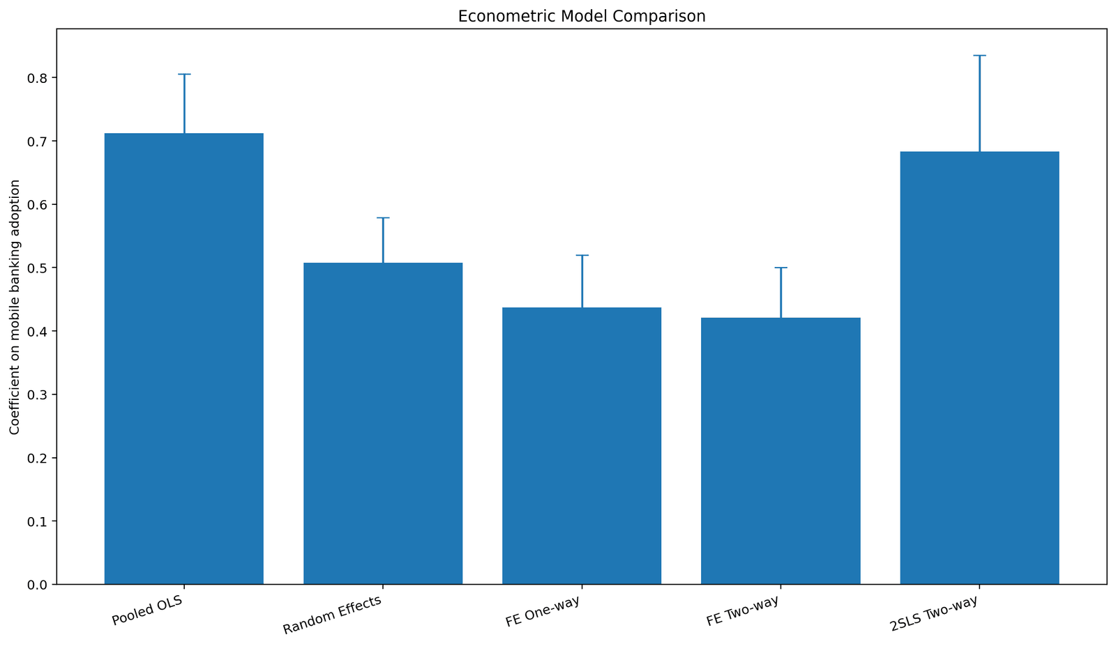
SpecificationCoefficientClustered SEWithin R²
Pooled OLS0.7120.0940.518
Random effects0.5080.0710.361
Fixed effects, one-way0.4370.0830.294
Fixed effects, two-way0.4210.0790.311
2SLS, two-way0.6830.1520.287

Coefficients are index points per percentage point of adoption. Under the preferred two-way fixed effects specification, a ten point rise in adoption corresponds to a 4.2 point gain on the inclusion index. Instrumented, that rises to 6.8 points, significant at 1%.

The IV correction runs the wrong way, and that is the interesting part. If endogeneity ran mainly through unobserved local demand, instrumenting would have pulled the coefficient down. It went up. That points to classical measurement error in self-reported adoption as the dominant problem rather than omitted variables, and it means attenuation was hiding roughly a third of the effect. Work in this literature that finds a positive association and stops there is usually assumed to be overstating. Here it was understating.

The average hides three patterns.

Rural units gain more. Interacting adoption with rural share gives 0.31 on the interaction. A unit at the 75th percentile of rural share sees an effect about 1.7 times that of a unit at the 25th. Where the nearest branch is far, a mobile account substitutes for something that was not practically available.

Low-baseline units gain more. Units starting below the median show 0.58 against 0.29 for units above it. That is convergence, not the divergence a pure payments-rail story predicts.

Agent density gates everything. Below roughly eight agents per ten thousand adults, the adoption coefficient is 0.11 and not distinguishable from zero. Above it, 0.52. A spline with a knot at the estimated threshold beats the linear form on both AIC and BIC.

What survives every specification. Adoption and inclusion are not the same thing, and the gap between them is a function of physical agent infrastructure rather than handset penetration. Results hold under Driscoll-Kraay errors, excluding Burundi, excluding the 2020 and 2021 waves, under an equal-weighted index, and under system GMM treating adoption as predetermined. The threshold moves between 7.4 and 9.1 across those variants, which is a range rather than a point, but not one that changes the conclusion.

Where that lands for policy. Licensing regimes that make agent operation viable in thin rural markets do more on this evidence than subsidies aimed at devices or data. A country reporting high registered-account figures alongside a sparse agent network may be reporting adoption without inclusion.

What it does not claim. The instrument is defensible rather than airtight; ruggedness could reach financial behaviour through market access, and Hansen J has limited power with two instruments. Ten years is short for savings and credit behaviour. And an increase in the inclusion index is not an increase in welfare. Easier access to short-term credit could run the other way for some households.

Gallery

Inside the Project

Ecometric model comparisons
Keep Exploring

More Case Studies

View all case studies →